Tracker Positioning Accuracy Analysis of Error Sources and System Limitations (And How to Improve It)

Positioning accuracy stands as the most critical performance metric for GPS trackers—and also the aspect most question raising by end users.  

"Why does the reported location drift across the street?" 

"Why does a stationary vehicle appear to be moving slowly?" 

"Why is the location fixed instantly sometimes, while at other times I have to wait a long while?"

These issues do not stem from tracker malfunctions, but rather are dictated by the inherent physical characteristics and system limitations of GPS technology.  This article delves deeply into the 12 primary sources of positioning errors, explains why these errors are difficult to completely eliminate, and presents a systematic framework for improvement—ranging from hardware selection to algorithm optimization.

Ⅰ. Basic Concepts of Positioning Accuracy

1.1 How positioning accuracy is measured

Before discussing positioning errors, we first need to understand how positioning accuracy is measured.

Simply put: under open skies, a tracker rated at "2.5 meters CEP" means that, over the long term, half of its positioning errors fall within 2.5 meters, while the other half exceed 2.5 meters. This represents the median value, not the maximum.

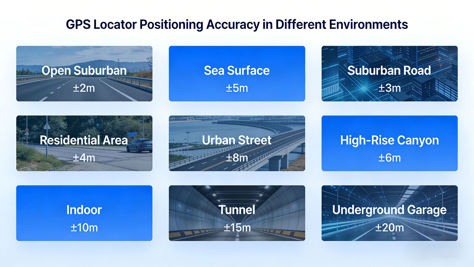
1.2 Typical Accuracy Under Different Environments

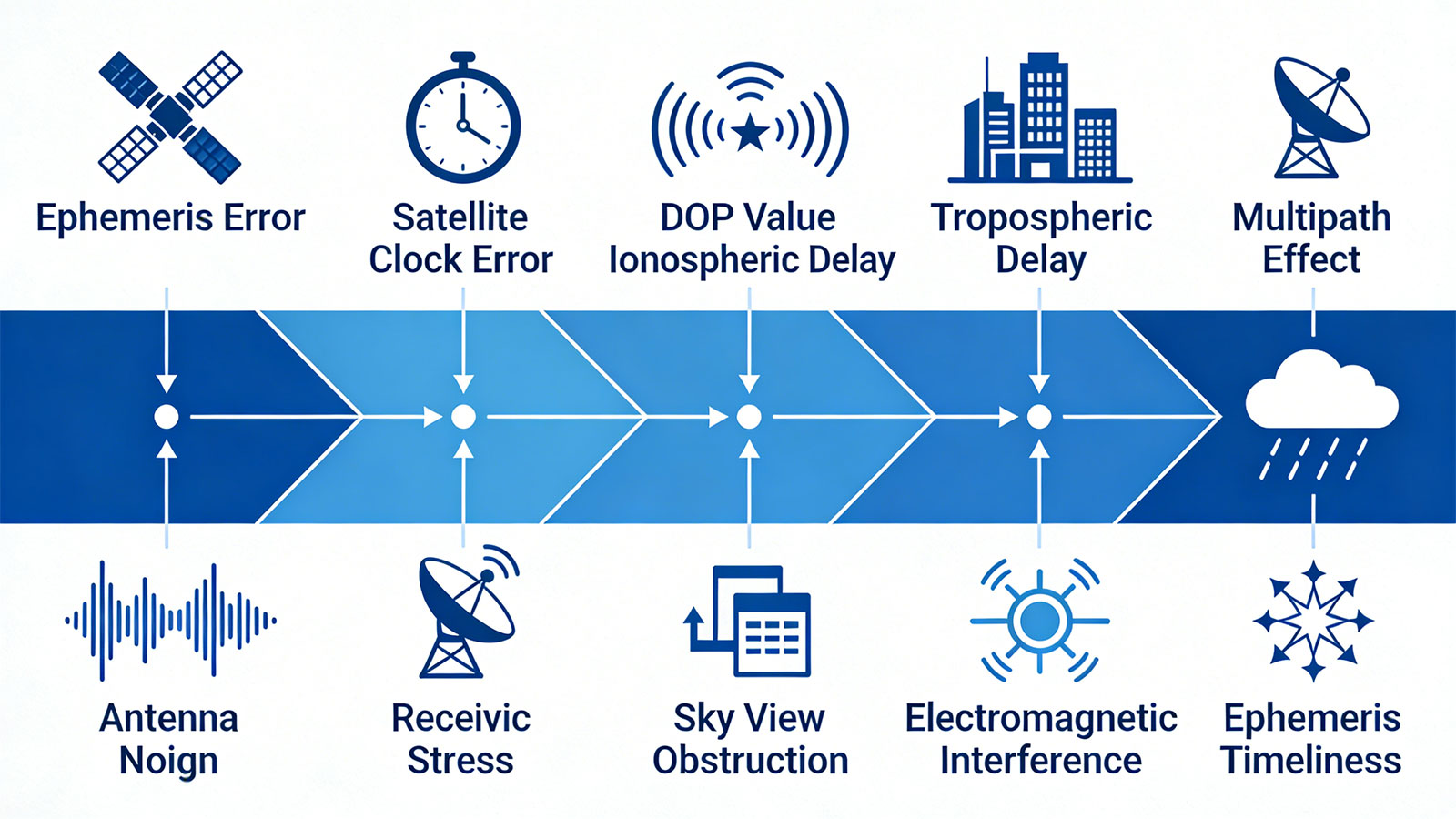
Ⅱ. Comprehensive Analysis of Sources of Error

2.1 Satellite-Side Errors

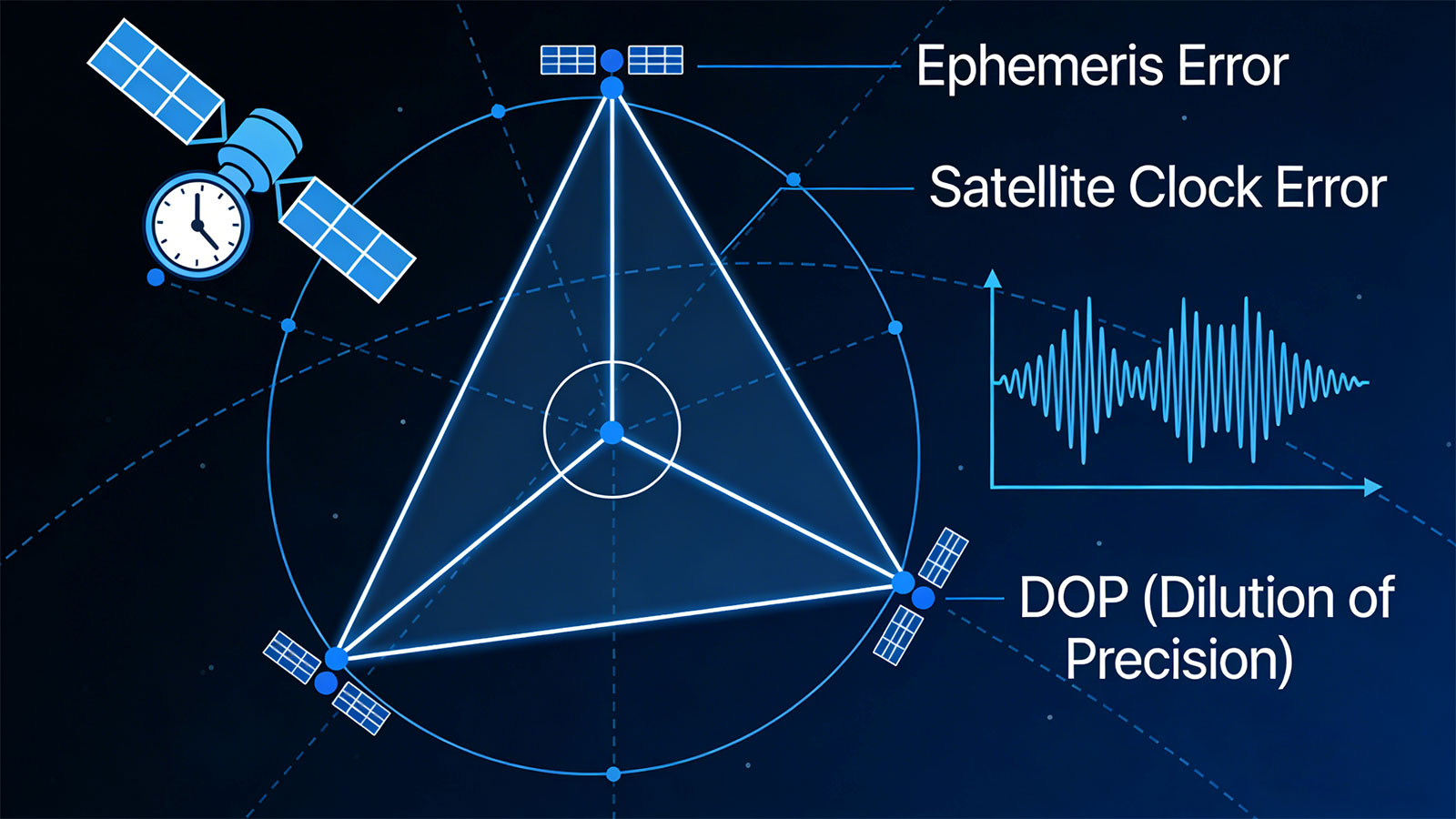
(1) Ephemeris Errors

GPS satellites do not orbit along absolutely precise trajectories. Influenced by factors such as the Earth's non-uniform gravitational field, solar radiation pressure, and lunar gravity, the satellites gradually deviate from their predicted orbits. Although the ground control system updates the ephemeris daily, minute errors still persist.

• Error Contribution: Approximately 1–2 meters

• Characteristics: All devices utilizing the same satellite share this error.

(2) Satellite Clock Error

Satellites are equipped with atomic clocks; although their precision is extremely high (cesium clocks can achieve a precision of 10⁻¹³ seconds), minute drifts still occur. Ground stations monitor and broadcast clock correction parameters; however, residual errors persist even after correction.

• Error Contribution: Approximately 1–2 meters

• Characteristics: Varies slowly over time

(3) Satellite Geometric Distribution (DOP Value)

Even if the number of available satellites is sufficient, their spatial distribution is of critical importance. When satellites are clustered within the same section of the sky, the resulting positioning is akin to "pinching a ball between two fingers"—highly accurate in the fore-and-aft direction, but prone to drifting laterally.

DOP Value Reference:

• HDOP < 1: Excellent

• HDOP 1–2: Good

• HDOP 2–5: Moderate

• HDOP > 5: Poor

Error Contribution: Can amplify other sources of error by a factor of 2 to 10.

2.2 Signal Propagation Path Error

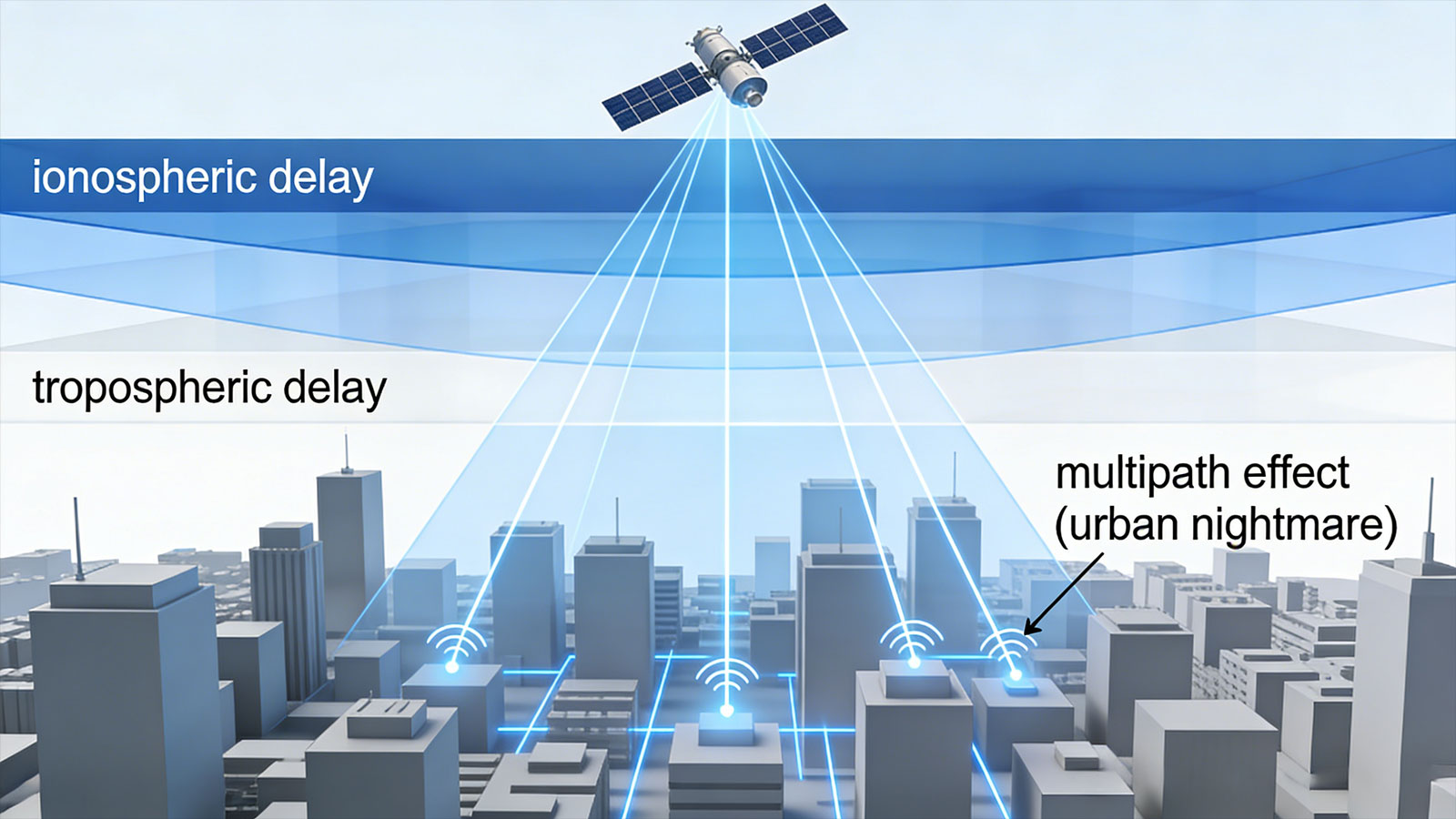
(4). Ionospheric Delay

When GPS signals traverse the ionosphere—located at an altitude of 60 to 1,000 kilometers above the Earth's surface—their propagation speed slows down. The magnitude of this delay depends on solar activity, time of day (day vs. night), and geographic location (equatorial vs. polar regions).

• Error Contribution: 5–15 meters (daytime), 2–5 meters (nighttime)

• Mitigation: Dual-frequency receivers can effectively eliminate this error.

(5). Tropospheric Delay

Water vapor and dry air within the troposphere (0–40 km above ground level) also delay signal propagation. Unlike ionospheric delay, tropospheric delay is frequency-independent and cannot be eliminated using dual-frequency techniques.

• Error Contribution: 2–5 meters (depending on humidity and elevation angle)

• Optimization: Model-based corrections can reduce the error by 70%.

(6). Multipath Effect (The Nightmare of Urban Environments)

GPS signals undergo reflection when encountering high-rise buildings, bodies of water, or metal billboards. Since the receiver simultaneously receives both direct and reflected signals—and is unable to distinguish between them—the calculated position deviates from the actual location.

• Error Contribution: 10–50 meters (potentially exceeding 100 meters in severe cases)

• Typical Manifestations: The plotted trajectory "jumps" to the side of an elevated bridge while driving underneath it; the reported position continuously "jumps" or drifts while a vehicle is parked next to a building with glass curtain walls.

• Optimization Difficulty: Extremely high; requires the synergistic coordination of both hardware and algorithms.

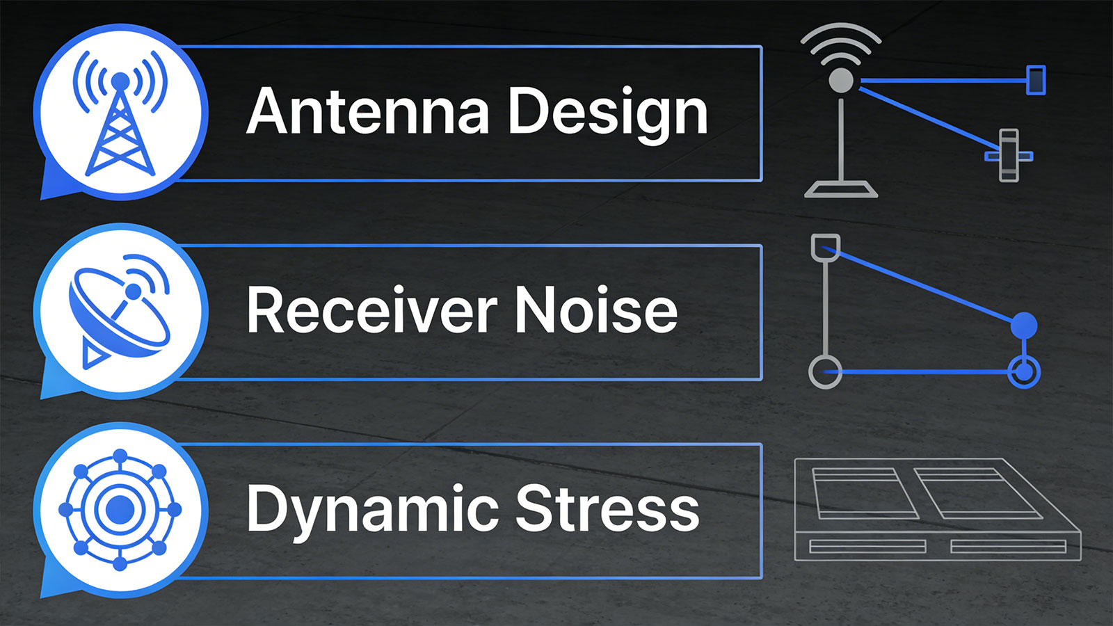
2.3 Receiver-Side Errors

(7). Antenna Design

The antenna serves as the "ears" of the GPS system. A poorly designed antenna can lead to:

• Non-uniform gain patterns (weak signals in certain directions)

• Unstable phase centers (inconsistent signal arrival times from different directions)

• Poor multipath rejection capabilities

(8). Receiver Noise

All electronic components generate thermal noise, which affects the precision of signal processing. High-quality receivers utilize lower-noise amplifiers and more sophisticated analog-to-digital converters.

• Error contribution: 0.5–2 meters (depending on receiver quality)

(9). Dynamic Stress

When a device is moving at high speeds (>100 km/h), the Doppler effect causes shifts in signal frequency. The receiver must track these frequency changes in real time; if processing power is insufficient, signal lag or abrupt jumps may occur.

• Error contribution: Particularly pronounced during rapid acceleration or braking 

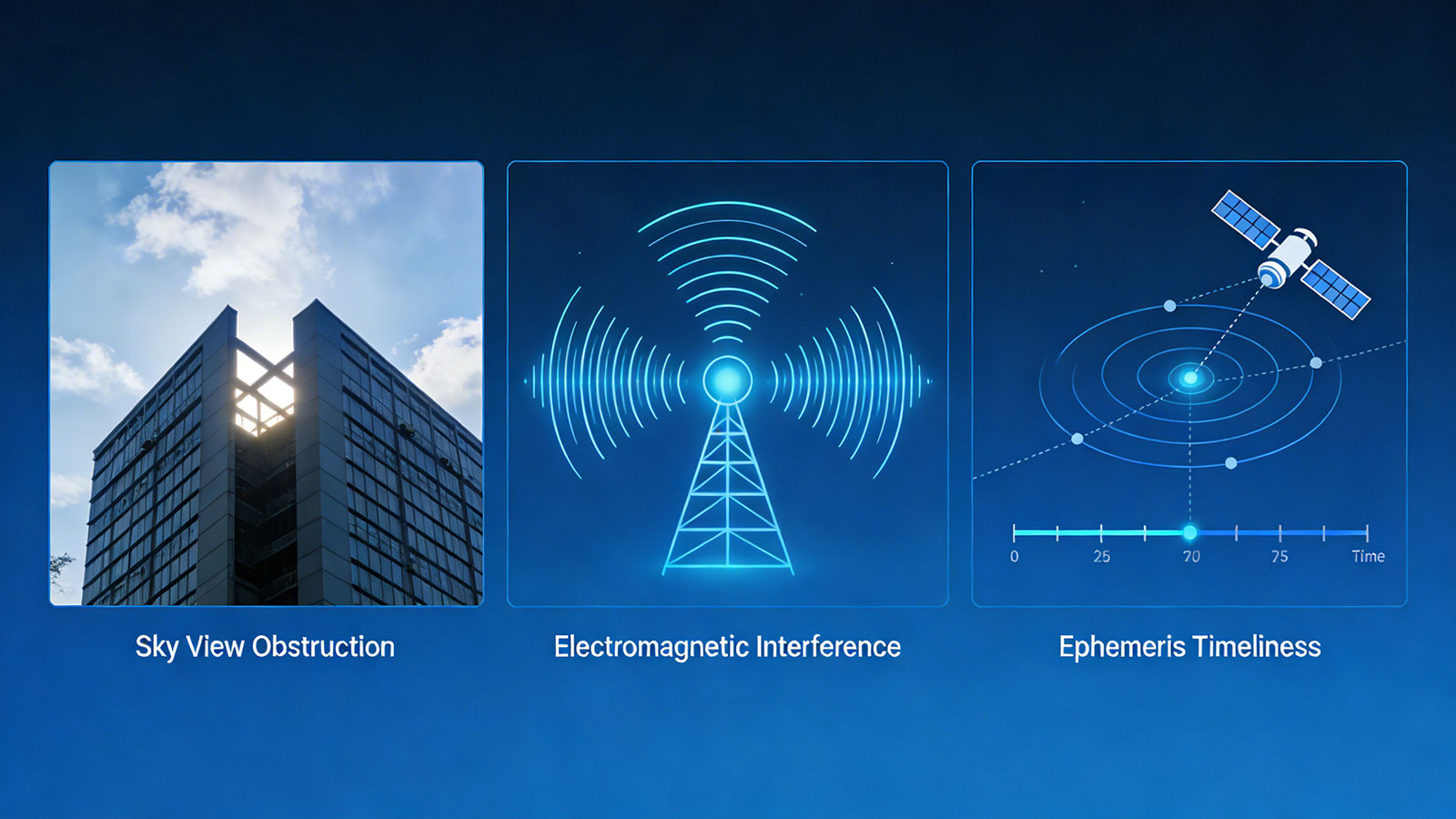
2.4 Environmental and Usage Factors

(10). Sky Visibility Obstruction

GPS signals cannot penetrate solid objects. Overhead foliage, tall buildings on either side, and metal vehicle roofs can significantly impact the number of available satellites and signal quality.

Impact of Obstructions:

• Dense foliage: Signal attenuation of 5–15 dB

• Single-pane glass: Attenuation of 1–3 dB

• Metal vehicle roof: Complete shielding

• Human body obstruction: Attenuation of 10–20 dB

(11). Electromagnetic Interference

Electromagnetic radiation originating from vehicle ignition systems, high-power electric motors, and radio transmission equipment may interfere with GPS signal reception.

• Typical Scenarios: When the electric motor in a new energy vehicle starts up, or when in the vicinity of high-voltage power lines.

(12). Ephemeris Timeliness

As discussed in our article "GNSS Cold Start, Hot Start, and Warm Start: Why Your Tracker's First Fix Time Varies from Seconds to Minutes?" ephemeris data remains valid for a period of 2 to 4 hours. Devices that are powered back on after a prolonged power outage must re-download the ephemeris data; during this process, positioning accuracy may be compromised.

Ⅲ. System Limitations: Why Is 100% Accuracy Unattainable?

Once the sources of error are understood, it is not difficult to see why GPS cannot achieve "absolute accuracy." These limitations represent the boundaries of physics and technology.

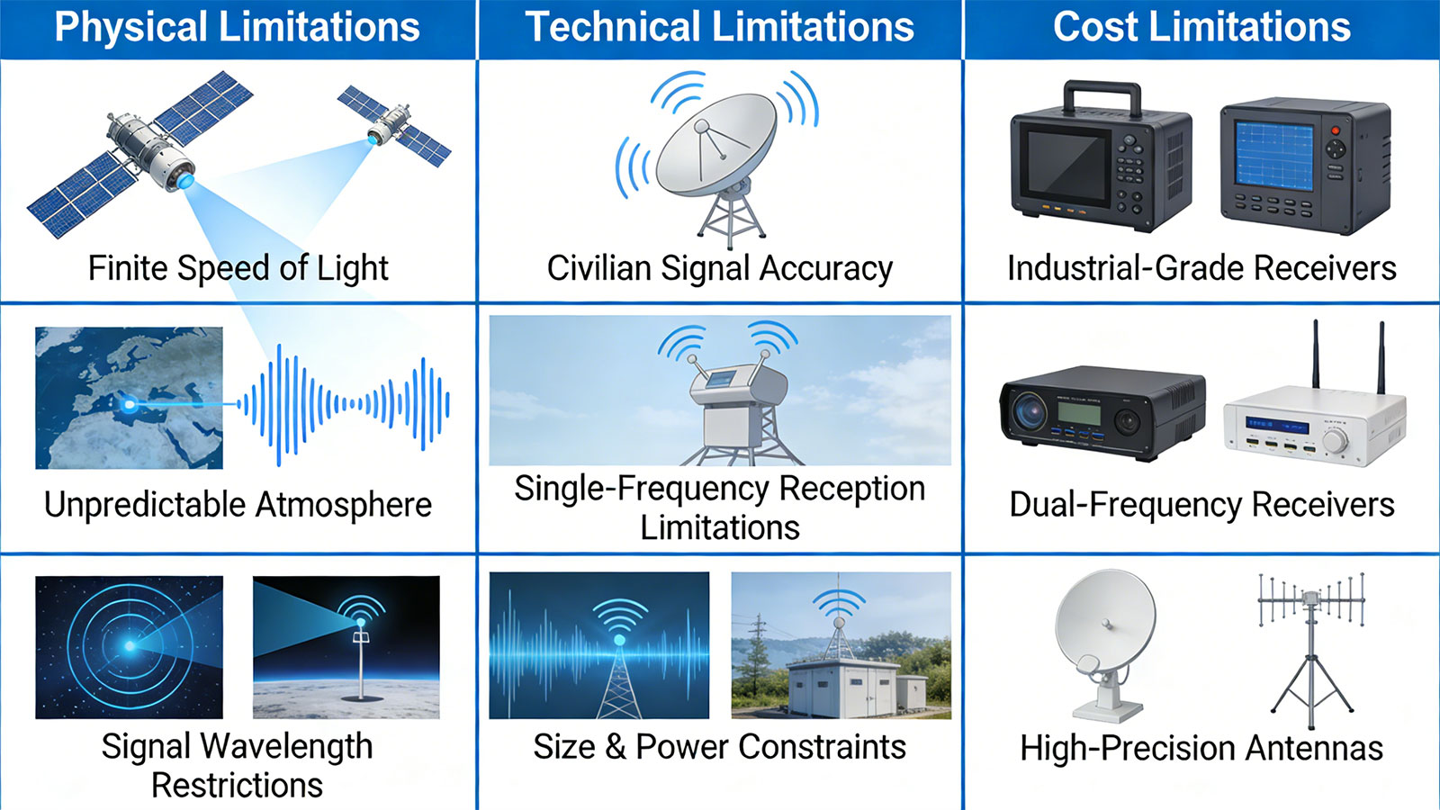
3.1 Physical Limitations

• Finite Speed of Light: In signal propagation time measurements, an error of 1 nanosecond (one-billionth of a second) corresponds to a distance error of approximately 30 centimeters.

• Unpredictable Atmosphere: The ionosphere and troposphere are dynamically changing environments; no model can completely eliminate their effects.

• Signal Wavelength Limitations: The wavelength of GPS signals is 19 centimeters (L1 band); theoretically, it is impossible to achieve a level of precision that exceeds this wavelength limit.

3.2 Technical Limitations

• Civilian Signal Accuracy: Although the U.S. government discontinued the Selective Availability (SA) policy in 2000, fundamental differences in accuracy between civilian and military signals persist.

• Single-Frequency Reception Limitations: Most consumer-grade devices utilize single-frequency (L1) reception; unlike dual-frequency receivers, they are unable to directly measure and eliminate ionospheric delays.

• Size and Power Consumption Constraints: High-precision positioning necessitates larger antennas, greater computational power, and higher energy consumption—requirements that conflict with the demand for lightweight, slim, and long-lasting portable devices.

3.3 Cost Constraints

• Industrial-grade receivers cost 3 to 5 times more than consumer-grade ones.

• Dual-frequency receivers cost 2 to 3 times more than single-frequency ones.

• High-precision antennas can be more expensive than the entire device itself.

In B2B business applications, it is essential to strike a balance among precision, cost, power consumption, and size, rather than blindly pursuing absolute maximum precision.  Looking for a suitable GPS tracker?  Please review the article: GPS Tracker Classification and Selection Guide: How to Choose the Right GPS Tracking Device for Your Solution?

Ⅳ. Methods for Optimizing Positioning Accuracy

Although position errors cannot be completely eliminated, we can keep them within an acceptable range through the application of systems engineering methodologies.

4.1 Hardware-level Optimization

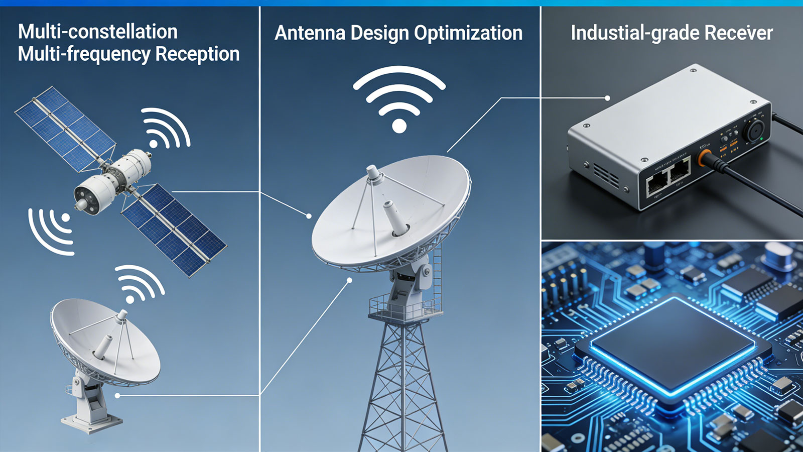
4.1.1 Multi-Constellation, Multi-Frequency Reception

• Multi-Constellation: Simultaneous reception of GPS, BeiDou, GLONASS, and Galileo; increases the number of available satellites by 40–60%, significantly improving performance in "urban canyon" environments.

• Multi-Frequency: Dual-frequency receivers can measure and eliminate ionospheric delay, reducing this error component from 5–15 meters to less than 1 meter.

4.1.2 Optimized Antenna Design

• Active Antenna: Features a built-in LNA (Low Noise Amplifier) to compensate for feedline loss.

• Right-Hand Circular Polarization (RHCP) Design: Better matches the polarization of GPS signals.

• Ground Plane Design: Suppresses multipath signals.

4.1.3 Industrial-Grade Receiver (If necessary)

• Higher Sensitivity (-167 dBm vs. -162 dBm)

• More Channels (50–72 channels vs. 22–32 channels)

• Built-in Multipath Suppression Algorithms

4.2 Algorithmic-Level Optimization

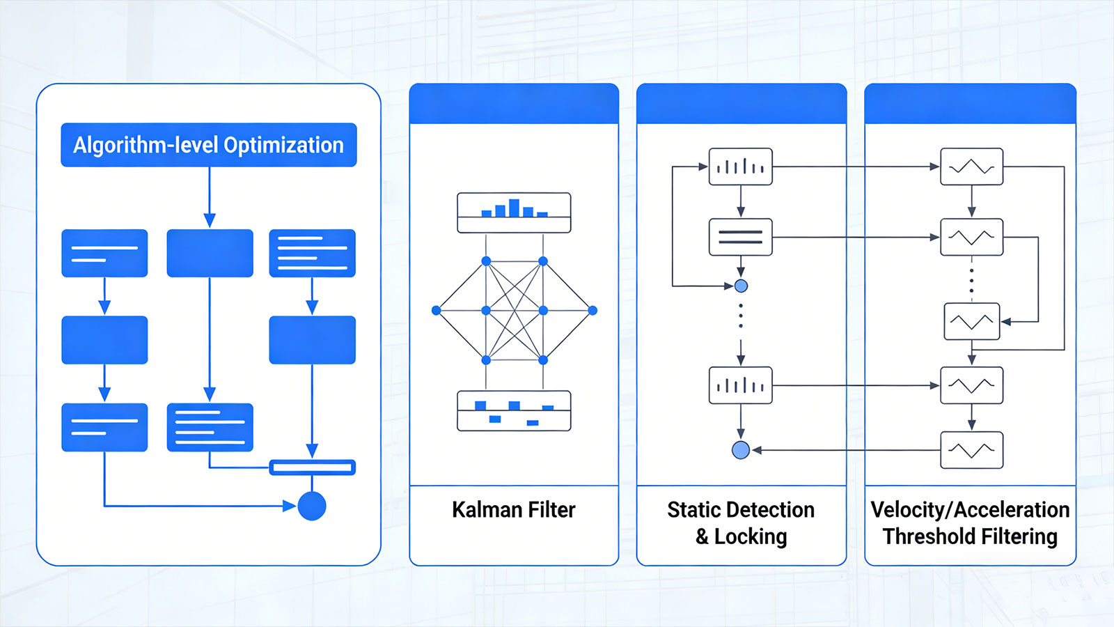
4.1.1 Kalman Filtering

Integrates historical trajectory data with current observations; it predicts the current position based on a motion model (e.g., constant velocity or constant acceleration) and performs a weighted average with GPS readings to effectively smooth out sudden positional jumps.

• Effect: Reduces static drift by over 70%.

• Implementation: Model parameters must be adjusted according to the specific application scenario (e.g., vehicles, personnel, or assets). 

4.1.2 Static Detection and Locking

Utilizes an accelerometer to determine whether the device is stationary. When stationary, the position is fixed—preventing any updates—thereby completely eliminating static drift.

• Effect: The reported position no longer "dances" or wanders while the device is parked.

• Note: Requires the use of a sufficiently sensitive motion sensor.

4.1.3 Velocity/Acceleration Threshold Filtering

Filters out implausible positional changes based on physical laws:

• Maximum velocity limit (e.g., a car not exceeding 200 km/h)

• Maximum acceleration limit (e.g., preventing instantaneous jumps of 100 meters)

• Direction change limit (e.g., preventing repeated U-turns within a 30-second interval)

4.3 System-Level Optimization

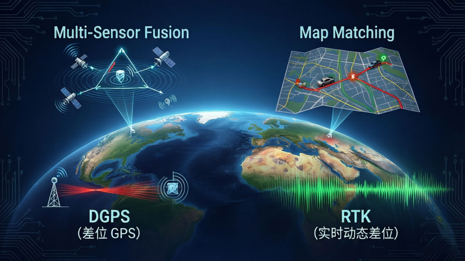
4.3.1 Multi-Positioning Technology

Fusion Logic: Prioritize high-precision sources; automatically fall back to lower precision when accuracy is insufficient, ensuring that "having a position is always better than having no position."  What is different for each type positioning technology?  Check Section of No.7 on article: How Does GPS Tracker Works?

4.3.2 Map Matching

"Snaps" raw trajectory points to the nearest road segments, eliminating off-road outliers caused by signal drift.

• Effect: The trajectory more accurately reflects the actual travel path.

• Limitations: May result in incorrect matching during off-road driving.

4.3.3 Differential GPS (DGPS)

Utilizes a reference station at a known location to calculate error correction values, which are then transmitted to a mobile station via a cellular network.

• Effect: Accuracy is enhanced to the sub-meter level.

• Applicability: Professional applications requiring extremely high precision. 

4.3.4 Real-Time Kinematic (RTK)

Utilizes carrier-phase measurements to achieve centimeter-level accuracy.

• Performance: 2–5 cm accuracy

• Applications: Autonomous driving, precision agriculture

• Cost: High receiver cost; requires the deployment of base stations or the use of network RTK services

4.4 User-Side Optimization

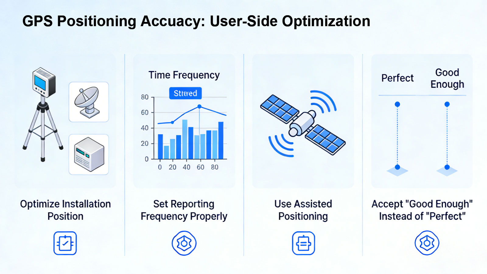
4.4.1 Optimize Installation Location

• Vehicle Trackers: Ensure the antenna faces upward and is positioned away from metal obstructions (e.g., do not hide it inside a metal trunk).

• Personal Trackers: Avoid deep pockets or internal backpack compartments; instead, place the device as close as possible to the outer surface of the body.

• Asset Trackers: Select a location where the top of the device is not covered by metal.

4.4.2 Set Reporting Frequency Appropriately

While high-frequency reporting enhances real-time responsiveness, it also introduces more data noise. In scenarios where absolute precision is not critical, slightly lowering the reporting frequency can yield a more stable and consistent tracking trajectory.

4.4.3 Utilize Auxiliary Positioning

In indoor environments or densely built-up urban areas, enable Wi-Fi or Bluetooth-assisted positioning. Our platform will automatically fuse data from multiple sources to enhance overall system reliability and usability.

4.4.4 Accept "Good Enough" Over "Perfect"

For the vast majority of enterprise applications, a positioning accuracy of 5–10 meters is sufficient to support effective business decision-making. Focus on the overall trajectory trends, dwell times, and zone entry/exit events, rather than fixating on the precise coordinates at any single point in time.

Ⅴ. Accuracy Requirements and Optimization Recommendations for Different Application Scenarios

Ⅵ. Conclusion: The Truth About Positioning Accuracy

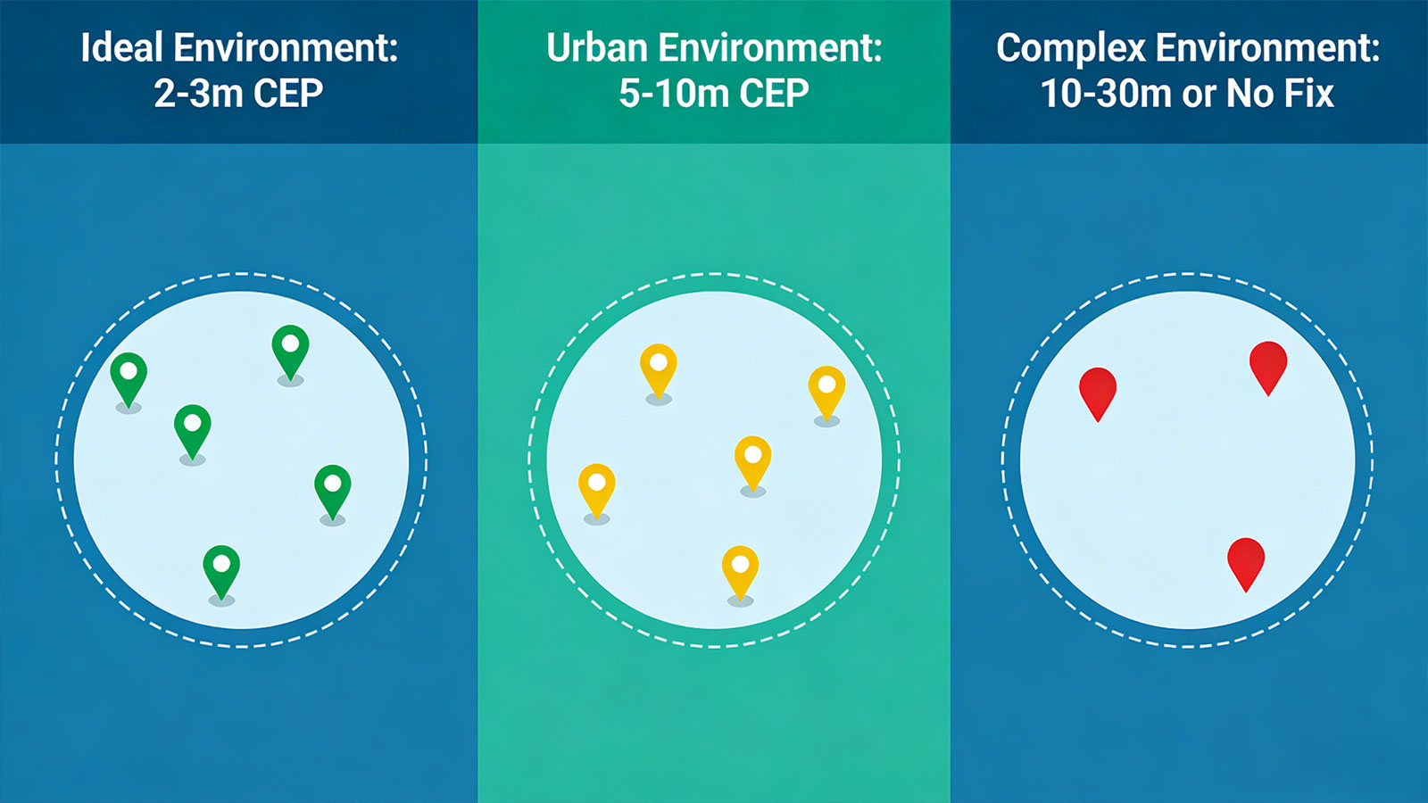
GPS positioning accuracy is not a fixed value, but rather a probability distribution that changes dynamically with the environment. Understanding this is a prerequisite for the rational design of IoT tracking solutions.

• Ideal Environment: 2–3 meters CEP

• Urban Environment: 5–10 meters CEP

• Complex Environment: 10–30 meters, or unable to obtain location

As an enterprise client, your focus should be on:

• The performance of the equipment within your actual deployment environment, rather than laboratory data;

• The vendor's engineering optimization capabilities (antenna design, algorithmic proficiency, and multi-source fusion);

• How the platform processes and presents imperfect raw data (map matching, trajectory smoothing, and confidence interval visualization).

Huaten Global's value lies not in manufacturing an “absolutely accurate” GPS—which is physically impossible.  Our value lies in:

• Deeply understand the optimal balance point between the technical limitations of GPS and specific business requirements.

• Through continuous optimization across hardware, algorithms, and system architecture, keep instances of "inaccuracy" within a range that is acceptable for business operations.

• Provide clients with transparent accuracy specifications and configuration tools, enabling location data to truly serve as a foundation for business decision-making.

If you have higher requirements for positioning accuracy in specific scenarios, we invite you to contact our solutions team. We can arrange prototype testing to evaluate and optimize positioning performance within your actual deployment environment.